While IoT data provides visibility, and in many instances real-time visibility, the real value of the visibility is harnessed by analytical approaches that are leveraged on this data. IoT data can be combined with other analytical areas as well to build unique and innovative solutions. One such area is geospatial analytics. Combining geospatial data with IoT data can help build innovative solutions and help address unique business problems.
In this article, we explore this intersection with an example.
Imagine that your company sells a device that measures airborne pollutants. It is internet-enabled and reports data back to your company regularly using MQTT. The target market for this product is environmentally-minded consumers who want to measure pollutants near their homes and contribute to the collective monitoring of the environment.
The value proposition is that they get free analysis of their local air quality in exchange for donating their data to support a cause they probably believe in anyway. Your company is planning to aggregate and package analytics of high-quality air pollution data to sell it to government and private organizations.
Since the device is sold to consumers indirectly through various retail outlets, your company is not initially aware of the location of the devices. The consumer connects the device to the internet and enters their addresses after purchasing it. At this point, the site can be determined.
The device has multiple sensors that measure the level of different contaminants in the air. One of the sensors measures the level of nitrogen dioxide (NO2). NO2 is a toxic gas and has even more damaging side effects. It facilitates the creation of acid rain and photochemical smog and is a precursor to other harmful secondary air pollutants such as ozone.
The burning of fossil fuels produces NO2. The main contributor in urban areas is typically motor vehicle exhausts, but the gas can also come from power plants, manufacturing facilities etc.
Your company wants to build and sell a data package summarizing NO2 levels by distance from Interstate highways. It also intends to aggregate the resulting data by each of the congressional districts in the United States.
This task may seem daunting at first, as all you know about device locations is the address registered by the customers. The first thought may be a manual process of reviewing each device’s location on a map and categorizing it based on its distance to the nearest Interstate highway.
This would be labor-intensive and cost prohibitive when you have 500,000 devices. Thankfully, geospatial analytics can do this type of analysis efficiently. We will introduce several concepts, revisit this example, and show how it can be solved.
Section 1: Storing geospatial data
There are many ways to store geospatial data. Depending on your intended use, a filesystem format or a relational database may be the most appropriate. I will cover an introduction to both.
File formats
There are hundreds of file formats for storing geospatial data. The most common for vector data is ESRI shapefiles. A shapefile consists of multiple files with the .shp extension for the main file. Most geospatially-aware software and Python packages know to look for the other needed files when given the location of the .shp file.
GeoJSON is another human-readable storage format. It uses a defined JSON format to store vector data definitions as text. It is easily readable but can get large.
Another way to represent vector data, whether in a file or code, is using the Well-known text (WKT) and binary (WKB) formats. WKT is human-readable, while WKB is not. WKB offers significant compression in size, so it is often a good choice for database storage. It can be converted into WKT upon reading.
Raster data is commonly stored in the Tagged Image File Format (TIFF) (.tiff) files. It can also be held as ASCII grid files, but the file size is a concern. Some compressed formats exist, such as Multi-resolution Seamless Image Database (MrSID) with the .sid extension and Enhanced Compression Wavelet (ECW) with the .ecw extension.
Spatial extensions for relational databases
With spatial extensions, relational databases can support storing geometry data in database tables and perform geospatial functions. These are typically not part of the standard installation but can be enabled through administration settings or by installing software extensions.
Relational Database Management Systems (RDBMS), PostgreSQL, and MySQL support spatial functionality for open source. PostgreSQL is by far the most popular and is the most fully functional. When the spatial components are enabled for PostgreSQL, it is commonly called PostGIS. You will see the terms used interchangeably. PostgreSQL is a supported RDS option on AWS. The spatial extensions can be enabled, turning it into PostGIS.
Oracle (Spatial and Graph) and SQL Server are famous for closed-source RDBMS. Oracle is generally considered the most capable one. These are not the only options, as more and more databases support spatial data. Amazon Aurora, a MySQL-compatible managed RDS database on AWS, has added spatial support.
Storing geospatial data in HDFS
HDFS and Hive do not natively support spatial data types. All is not lost, though, as HDFS can store any file, including geospatial files. Geometry can be stored in string (WKT) and binary (WKB) forms. They can be converted using code upon retrieval. Hive tables are schema-on-read and support User Defined Functions (UDF). A UDF can be created to interpret geospatial data.
Some open-source projects do just that. One is called SpatialHadoop and can be found at http://spatialhadoop.cs.umn.edu/index.html. Another is called spatial-framework-for-hadoop and can be found on GitHub (https://github.com/Esri/spatial-framework-for-hadoop). The downside is that these projects are not fully supported or part of the Cloudera and Hortonworks Hadoop distributions.
A more robust method is to store spatial data as WKT or WKB and use geospatial Python packages to manipulate it.
Spatial indexing
Imagine trying to find where someone lives if you do not know their house address, postal code, or even their country. You would have to visit every home until you run into the person you are looking for, which will take longer than you have left and would not be very enjoyable anyway.
Thankfully, addresses allow quick identification of where someone lives by identifying the country, the state or province within that country, the zip code, and the street name where you can drive until you find their house number, which tends to follow an established order along the street.
Spatial databases can get very large, so an efficient method of searching for geometry is needed to improve response times. This is where spatial indexing comes into play. There are a variety of techniques that are employed to do this. We will cover one of the more popular methods next.
R-tree
R-tree is a spatial indexing method used in both PostGIS and Oracle databases. It leverages the bounding box concept to create a hierarchical index tree. The tree is balanced because all branches have the same level of nodes. We will walk through a simple example to understand how a primary R-tree index is built.
A spatial database such as PostGIS can quickly create an index on a geometry field. A simple SQL statement such as the following for PostGIS will build an R-tree index. PostGIS builds it on a Generalized Search Tree (GiST) layer for robustness. GiST is a generic algorithm that can be used with several indexing methods.
Note: A Python package called tree can also be used to build an index as part of a code module. This can be useful for some heavy-duty geospatial processing where you must repeatedly scan through a set of geometries.
Section 2: Processing geospatial data
Specialized software can help in processing and visualizing geospatial data. This can be useful for small data and one-time analyses. Even if you have a big data solution, using these tools can help you communicate your findings more effectively to others.
Geospatial analysis software
I will introduce the most popular Geographic Information System (GIS) tools so you have some familiarity with them. They are helpful support tools for geospatial analytics.
ArcGIS
ArcGIS is the de facto standard for paid GIS software. It was developed and maintained by the ESRI corporation. It has an awe-inspiring amount of functionality and is used by most professional geospatial analysts. It has world-class support from ESRI, and many training options abound. It links to valuable datasets and geospatial analytic capabilities, also maintained by ESRI.
ArcGIS is available as a desktop application or as a cloud service. You can sign up for a 60-day free trial (https://www.arcgis.com/features/free-trial.html). You can use ArcGIS for various analytics, including geocoding your custom shapefile.
QGIS
QGIS is open-source and very powerful desktop GIS software. It is similar to ArcGIS but not to the full scope of capability as the paid ESRI software. But the price is right, and it still has various capacities. It can also be manipulated with Python code. There is a vast trove of documentation on it and many valuable books on how to use it.
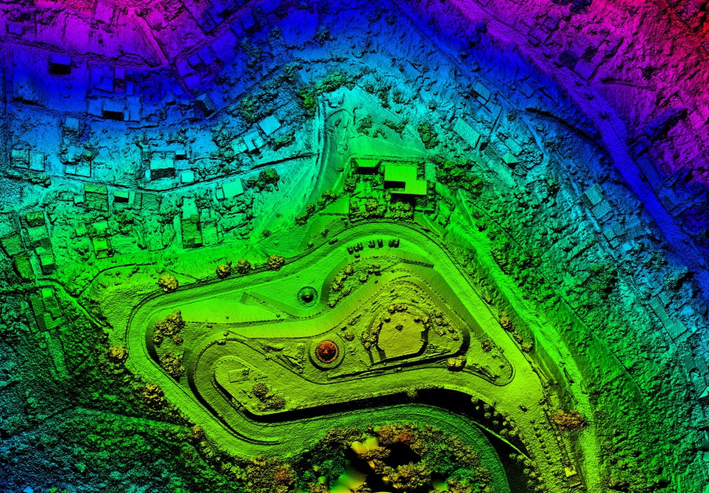
You can download and install QGIS from the project site http://www.qgis.org/en/site/forusers/download.html. If you are unable to get ArcGIS, make sure to keep QGIS handy. QGIS was used to create many of the images in this book. You can connect both QGIS and ArcGIS directly to geospatial databases, such as PostGIS and Oracle. The following image shows an example of what can be created with QGIS:
ogr2ogr
ogr2ogr is part of the GDAL library. It is a command-line tool that converts files from one OpenGIS Simple Features Reference Implementation (OGR) spatial format to another. It is a no-frills tool but is used heavily by geospatial analysts. The general format for a command-line conversion follows the following example:
ogr2ogr -f “file_format” destination_data source_data
For example, you can use it to convert PostGIS data into shapefiles or load shapefiles into PostGIS. It supports conversion into over 90 file formats for vector data alone.
PostGIS spatial functions
PostGIS contains dozens of spatial functions that can be referenced in a standard SQL query. The following table provides an overview of some commonly used functions:
| Function | Description |
| ST_GeomFromText | This returns a specified ST_Geometry value from the WKT representation. |
| ST_GeomFromWKB | This creates a geometry instance from a WKB geometry representation and optional SRID. |
| ST_Buffer | This returns a geometry covering all points within a given distance from the input geometry. |
| ST_ConvexHull | The convex hull of a geometry represents the minimum convex geometry that encloses all geometries within the set. |
| ST_Intersection | This returns a geometry that represents the shared portion of geomA and geomB. |
| ST_Simplify | This returns a simplified version of the given geometry using the Douglas-Peucker algorithm. |
| ST_Boundary | This returns the closure of the combinatorial boundary of this geometry. |
| ST_Transform | This returns a new geometry with coordinates transformed to a different spatial reference. |
| ST_Centroid | This returns the geometric center of geometry. |
| ST_ClosestPoint | This returns the 2-dimensional point on g1 that is closest to g2. This is the first point of the shortest line. |
| ST_Contains | This returns true if and only if no points of B lie in the exterior of A, and at least one point of the interior of B lies in the interior of A. |
| ST_Covers | This returns 1 (TRUE) if no point in geometry B is outside geometry A. |
| ST_Crosses | This returns TRUE if the supplied geometries have some, but not all, interior points in common. |
| ST_Distance | For the geometry, the type returns the 2D cartesian distance between two geometries in projected units (based on spatial ref). For geography, the type defaults to produce the minimum geodesic distance between two geographies in meters. |
| ST_Intersects | This returns TRUE if the geometries/geography spatially intersect in 2D – (share any portion of space) and FALSE if they don’t (disjoint). For geography, tolerance is 0.00001 meters (so any points that close are considered to intersect). |
| ST_Length | This returns the 2D length of the geometry if it is a LineString or MultiLineString. The geometry is in units of spatial reference, and the geography is in meters (default spheroid). |
| ST_Touches | This returns TRUE if the geometries have at least one point in common, but their interiors do not intersect. |
These functions can be used easily as part of a SQL query.
Geospatial analysis in the big data world
Volume and velocity pose some challenges for geospatial analytics. The data size can easily become too large to analyze with a desktop GIS tool. It could also be too large to handle effectively in a relational database with spatial extensions. Due to the intensive computational requirements of geospatial functions, near real-time response can also be a challenge.
Some options exist for geospatial analysis with tools explicitly built with big data in mind. Elasticsearch is an open-source distributed search engine. It can scale from one server to hundreds of servers and has some spatial search functions. For example, you can search for locations within a certain distance of a latitude and longitude point. AWS offers a managed Elasticsearch service where there is no need to worry about managing servers.
AWS also has a managed petabyte-scale data warehouse service called Redshift. Redshift does not support geometry fields directly but does support Python UDFs. You can create UDFs using Python code and the shapely package, then call them from Redshift SQL statements. A similar strategy can be used for both Hive and Spark.
ESRI supports an open-source project called GP tools for AWS that allows ArcGIS users to connect to Amazon EMR and S3 data sources. The project is hosted on GitHub (https://github.com/Esri/gptools-for-aws).
References:
- Chapter 7. PostGIS Reference. https://postgis.net/docs/manual-1.5/reference.html
- GIS functions – Apache Drill. https://drill.apache.org/docs/gis-functions/
- https://drill.apache.org/apidocs/org/apache/drill/exec/udfs/gis/package-summary.html
- http://spatialhadoop.cs.umn.edu/index.html
- https://github.com/Esri/gptools-for-aws
- http://www.qgis.org/en/site/forusers/download.html
- https://www.arcgis.com/features
