In the first part of the article, we reviewed the field of Deep Reinforcement Learning (DRL) and started exploring some fundamental terminology in the second and third parts. In the fourth part, we explored the temporal credit assignment problem, and the fifth part focused on the exploration vs. exploitation trade-off. In the sixth part, we explored the Markov decision process (MDP) and its role in reinforcement learning. We started exploring a detailed example in the seventh part that we continued in the eighth part. In the ninth part, we will explore the role of reward function.

We have iterated many times that one of the key assumptions of reinforcement learning algorithms is that the probability distribution is stationary. What this means is that while the transitions are highly stochastic, the probability distribution does not change during the algorithm training and evaluation. In our frozen lake environment example, we know that there is a 33.3% chance of transitioning to the intended state and a 66.6% chance that instead of transitioning to the intended state, we end up transitioning to orthogonal directions. And then there is also the probability that we will bounce back to the previous state if that previous state was next to a wall. Note that an action, and a resultant state, may have an associated reward.

The reward function maps a transition to a scalar value. We know that the tuples of a transition R are action, current state and new state. The reward function maps these variables to a scalar value which acts as a numerical signal of the goodness of the transition. A positive signal or a positive reward indicates that the transition has yielded good results. As you can imagine, most problems have a minimum of 1 positive signal. An example is winning the game of checkers.

While common sense dictates that reward should be always positive, that is not necessarily always the case. Rewards can be negative too, we just then would call them something else in the real world, like penalty. If we go back to the warehouse bot example that we discussed in the very first part of this article series, adding a time step penalty is leveraged widely in robotics. The rational is that while the bot definitely wants to reach an end state, it wants to do that in a minimum number of time steps possible. An aspect that we need to keep in mind, in the parlance of reinforcement learning, is that irrespective of whether the value is positive or negative, the scaler value gets generated by the reward function, is always referred to as the reward. That is why we indicated that reward function can be negative too.

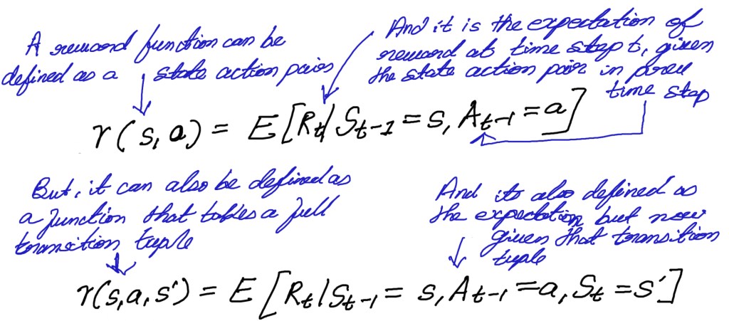
Like transition function, we can represent the reward function through its variables R (s,a,s’). We can also use variations of the reward functions like R(s,a) or R(s), depending on the scenario. If we need to reward the agent based on state then we use R(s). Sometimes we may want to reward based on the action and the state and in that case we will use R(s,a) variant. But generally, the first approach of R(s,a,s’), that uses state, action and the next state, is the most widely leveraged way to represent the reward function. This approach allows us to calculate the marginalization over next states to obtain R(s,a) and then the marginalization over actions in a to obtain R(s). The mathematical representation of reward function has been shown below.

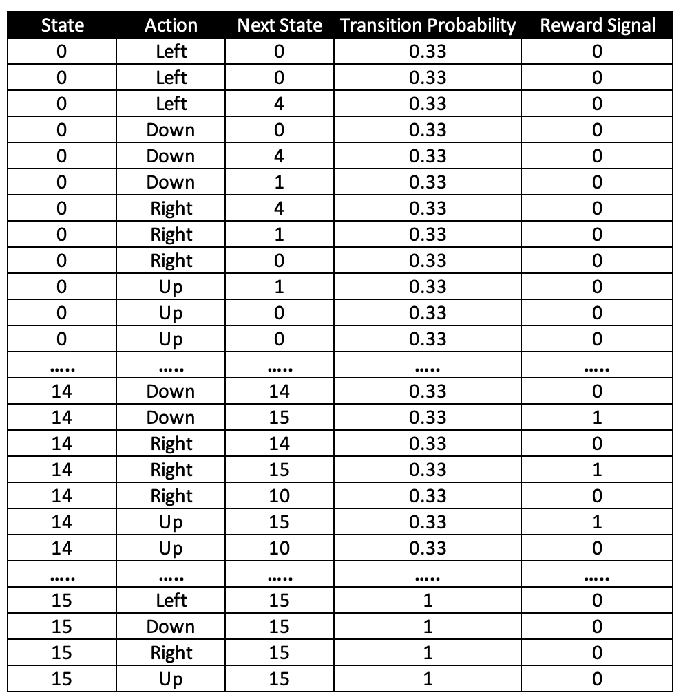
In our frozen lake environment, our reward function for landing in state 15 is +1. For all other moves it is 0. For example, if you are in 14, there are only three approaches to get to 15. First is that you choose the right action, with the intention to move to 15 and that action, with 33.3% probability, will land you in 15. The second and third approaches are that you may also end up choosing a wrong direction that does not lead to 15, but may still end up in 15 unintentionally since there is a probability of 66.66% of not landing in intended direction. A subset of the transition and reward function for our example has has been illustrated in the table below. Note that this is just an illustrative subset, not the full table.

In the next part we will discuss the role of time horizon and the concept of discounting reward value. The next part will be published on 08/05.