In the first part of the article, we reviewed the field of Deep Reinforcement Learning (DRL) and started exploring some fundamental terminology in the second and third parts. In the fourth part, we explored the temporal credit assignment problem, and the fifth part focused on the exploration vs. exploitation trade-off. In the sixth part, we explored the Markov decision process (MDP) and its role in reinforcement learning. We started exploring a detailed example in the seventh part that we will continue in this eighth part.

There are certain standard symbols used to denote certain environmental components and variables in reinforcement learning. S+ represents set of all states in the MDP. Si is the set of initial states or the starting states. To start interacting with an MDP, we define a state from Si, leveraging probability distribution. This distribution can be anything depending on the problem but the gist is that the distribution remains fixed throughout the training. This means that the probabilities must remain the same, starting from the first episode to the very last episode of training and for agent evaluation.

As discussed in the frozen lake environment in the last part of this article, our example environment has terminal states as well, also known as absorbing states. The set of all non-terminal states is represented by S. While generally you will see that there is only one terminal state in which all terminal transitions get absorbed, there may be environments which have multiple terminal states. A terminal state is one that should have a probability of one for all actions transitioning into it, and these transitions should not provide any reward. Note that we are discussing the transition from the terminal state, not to the terminal state.

In our frozen lake instance recall that we have one starting state which is the stage 0 and five terminal states which are basically the holes in the icy surface of the frozen lake 😁.

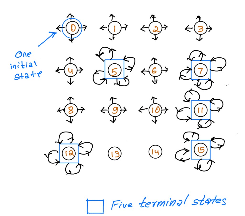
Errata: 13 and 14 should also have all directional arrows like all other non terminal states.

The set of actions that MDP’s make available into the environment is generally denoted by A. This set of actions that MDP makes available depends on the state. What this means is that certain actions that may not be allowed in one state, may be allowed in another state. The function of A takes a state as an argument A(s). The function returns the set of all available actions for the given state s. The only scenario where all actions are available at every state is when the states are constant across the state space. We can also prohibit an action in a given state by setting all transitions from a state action pair to 0.

The action space, like the state space, can be finite or infinite. However, the set of variables of a single action, though may contain more than one element, must be finite. Unlike the number of state variables, the number of actions variable may not be constant from one state to another. We already discussed the reason behind this. Actions that are available in one state may not be available in another state and hence actions variable differ from one state to another. However, for the sake of simplicity, most environments are designed in a way so that the number of actions remains the same in all states.

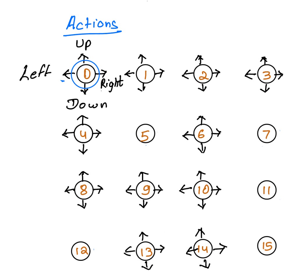
As we can imagine the set of all available actions is known in advance. The agent can then decide to select actions based on deterministic or stochastic analysis. Note that this does not mean that the environment reacts deterministically or stochastically to agents actions. The gist here is that agents can either select actions from a table or from pre-state probability distributions. In our frozen lake environment, actions are singletons representing the direction the agent tries to move to, which is four (up, down, left and right). So we can say that the number of variables for the action is just one, which is the direction of the move and the size of the action space is four (number of directions in which the agent can move).

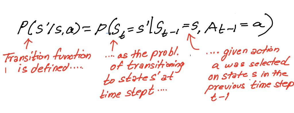
We know that an environment changes as a response to actions. The way this change is captured mathematically is known as state transition probabilities, or as we defined it more simply in one of the early parts of this article, the transition function.  The transition function is denoted by T(s,a,s’). It maps a transition tuple of s, a and s’ to a probability. What this means is that the transition function captures the following scenario: When you provide a transition function the current state s, the intended state s’ and the action a, it returns the probability of transitioning to state s’. The mathematical representation of the transition function is shown below.

The frozen lake environment in our example is stochastic. What this means is that the probability of the next state s’ , given the current state s and the action a, is less than one. A key assumption of many reinforcement learning algorithms is that this distribution is stationary. What this means is that while there may be stochastic transitions, the probability distribution may not change during the training or during evaluation. But as we did with Markov assumption, we often relax the stationarity assumption to a certain extent.

We will continue developing MDP for the frozen lake environment in the subsequent parts of this article. The subsequent part will be published on 08/03.