In the first part of the article, we reviewed the field of Deep Reinforcement learning and started exploring some fundamental terminology in the second and third parts. In the fourth part, we explored the temporal credit assignment problem, and the fifth part focused on the exploration vs. exploitation trade-off. In the sixth part, we explored the Markov decision process (MDP) and its role in reinforcement learning.

In the previous part, we mentioned that we will explore the Markov decision process further with an example. For our example, we will use the frozen lake (FL) environment, a simple grid-world environment in reinforcement learning. The task in this environment is simple. The objective is to go from a starting location to a final location while avoiding falling into holes. Just like our “slippery here to there” environment, the surface of a frozen lake is also slippery. The overall environment, however, is much larger, as shown in the figure.

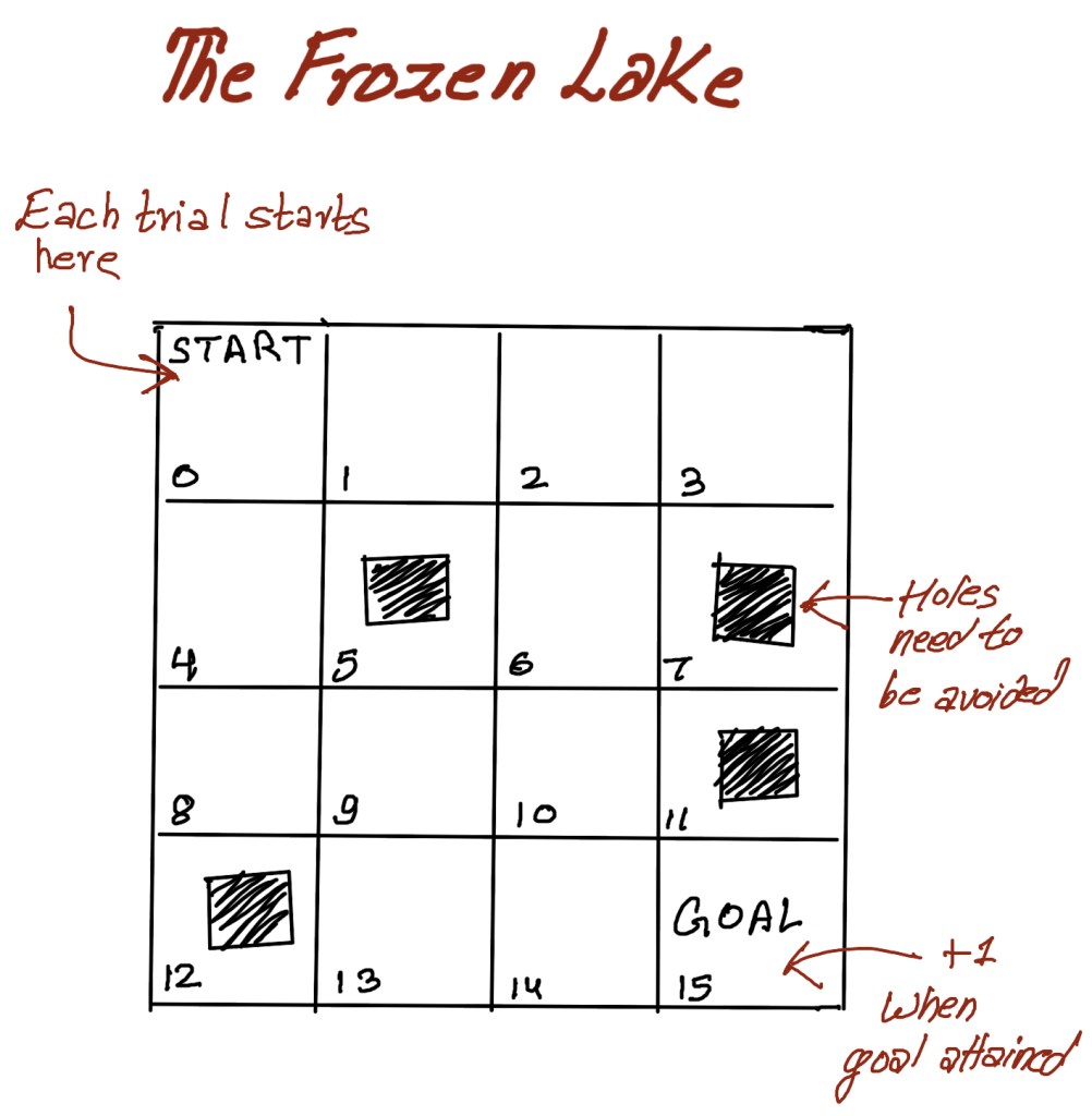
The environment is a 4 X4 grid. It has 16 cells. There is a START cell which is the cell 0 as shown in the figure. In every episode, the agent starts in the START cell. There is a reward of +1 for reaching the goal cell. Every other move is a net zero. Since the surface of the frozen lake is slippery (duh…. it’s a frozen lake!), the agent is successfully able to navigate in the intended direction only 1/3 of the time. For the remainder. That is 2/3 of the time, the agent may move evenly in orthogonal directions.

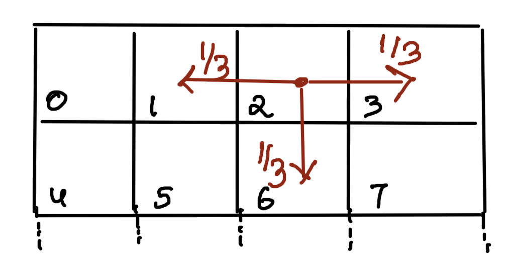
What this means is that if the agent decides to move right, then there is a 33.3% chance that it will be able to move right. The remainder of 33.3% and 33.3% pertain to the probability that it may move left or down respectively.

Also, the environment assumes that there is a fence around the lake to prevent the agent from moving out of the grid world. There are four holes in that ten eyes of the lake and the game terminates if the agent falls into one of the holes. We will now build the MDP for this problem.

Recall from the previous parts that a state of the environment is a specific, self-contained configuration of the environment or the problem. The state space is the set of all possible states. As you may have noticed, the state space is different from the set of variables that constitute a single state. So while the state space can be finite or infinite, a single state must always be finite and should be of constant size from state to state.For our frozen lake example the state comprises of a single variable, which is basically the idea of the cell, where the agent may be at any given point of time. The size of the state space is obviously 16 for this problem.

In MDPs, envorinments need to be fully observable . This means that we are able to look at the internal state of the environment at every time step . States must contain all the variables that are required to make them independent of all other states. In our frozen lake environment we only need to know the current state of the agent to predict predict its next possible states. So for example, if we know that the agent is in state 2, then we obviously know that the agent can only move to stage 1,3, 6 or 2, regardless of the previous state of the agent.

Hence, the probability of the next state given that we know the current state and the possible actions, is independent of the historical states, or the history of interactions. This memoryless behavior of MDP’s is known as the markov property. The probability of moving from one state as to another state, as on two separate occasions, given the same action a, is the same regardless of all previous states or actions encountered before that point.

The mathematical representation of the markov property has been shown below.

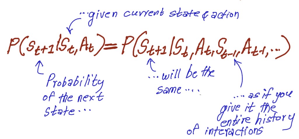
While you do not need to fret about the complexity of this, the key take away here is that because most RL and DRL agents leverage markov assumption, one of the most critical aspects to feed the agent is the variables that are necessary to make the agent hold to Markov assumption as tightly as possible. For example, if SpaceX is leveraging DRL to land its rockets, it’s agent must receive all the variables that capture velocities along with its locations. Locations alone, as you can assume, will not be sufficient.

But then what about velocity (in these SpaceX example) ? We know that acceleration is to velocity what velocity is to position. So if we go ahead and include acceleration, then some other variable also comes into play. So the question is, how far do you go to make the MDP purely Markovian? You have to keep in mind that completely forcing the Markov assumption is impractical and maybe impossible as well. To understand how deep you can go is a combination of art and science, which is beyond the realm of this article series, but to conclude this part, for our specific grid world environment, only the state ID location of the agent is sufficient.

In the next part, we will continue our journey of developing MDP for the frozen lake environment. The next part will be published on 08/02.