While in the first part of the article, we overviewed what the field of Deep Reinforcement learning is about, we started exploring some fundamental terminology in the second and third parts. In the fourth part, we explored the temporal credit assignment problem and the fifth part was focused on the exploration vs exploitation trade-off. In this part, we will explore Markov Decision Process (MDP) and its role in reinforcement learning.

We ended the fifth part of this article by stating that most real world decision making problems can be expressed as reinforcement learning environments and a framework that is frequently used to represent decision making process in reinforcement learning is known as Markov decision process.

A Markov decision process (MDP) is a stochastic decision-making process that uses a mathematical framework to model the decision-making of a dynamic system in scenarios where the results are either random or controlled by a decision maker, which makes sequential decisions over time, like the agent in our case. In reinforcement learning, we assume all environments have an MDP working behind them. You name any reinforcement learning problem, whether it is a self driving car or stock market optimization, they all have an MDP running behind them.

Let us try to understand markov decision process with the help of an example. We will use a simple grid world environment for our example. Grid worlds are a common type of environment for studying reinforcement learning algorithms.

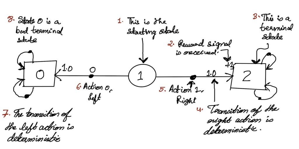
Let us name our environment as HT, which stands for here or there. It is a very simple environment with only three states and one of those states is a non terminal state. In the world of reinforcement learning environments that have a single non terminal state are generally referred to as bandit environments.

So our HT environment has just two actions available: a left action which we will call “here”, denoted by 0 and the right action which we will call “there”, denoted by 1. HT has a deterministic transition function which means “here” action always moves the agent to the left and “there” action always moves the agent to the right. The reward signal is plus one when the agent lands on the rightmost cell, otherwise it is 0. The agent starts in the middle cell. Now let us draw a graphical representation of the HT environment.

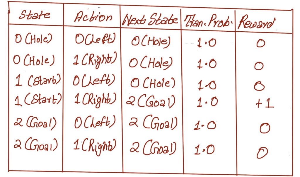
While a graphical view is always helpful, there is another way to represent the environment. That tabular form of representation has been shown in the table below

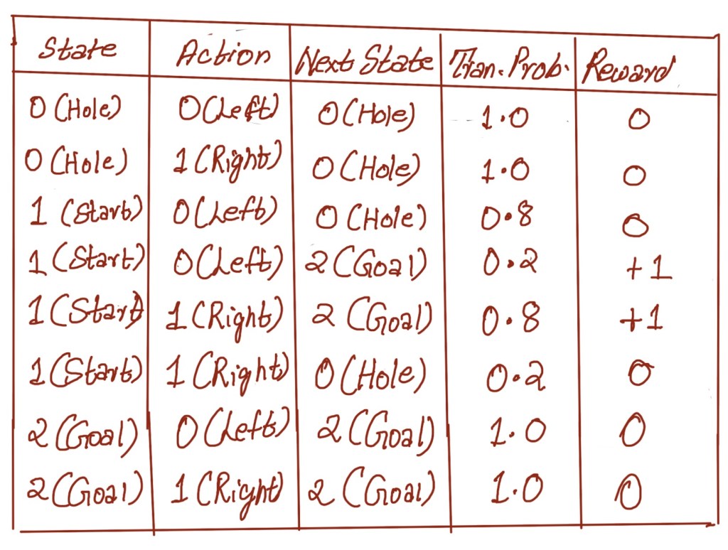
Now let us consider another example. Let us assume that the surface on which the agent walks gets oil spilled on it. So now each action has that 20% probability that the agent may slide backwards. We can call this new environment “slippery here and there” (SHT). But remember it is still one row grid world with only left and right actions available.

Just like our previous example, it has three states and two actions. The reward is same as well. However the transition function here is different since because of the oil the agent may slide and there is 20% probability of agent sliding backwards. Hence we can say that 80% of the time the agent move to the intended cell and 20% of the time slides back in the opposite direction. We can represent this environment in the form of a graph like the one below

Now let us capture the same environment in a tabular form like we did for the previous environment.

What we are essentially doing in these tabular representations is representing the environment in the form of markov decision process. This representation, though straightforward, is very powerful when it comes to developing models of complex sequential decision making problems under uncertainty. To represent the ability to interact with an environment in an MDP, we need states, observations, actions, or transition, and a reward function, as you can decipher from the table.

In the next part of the article, we will explore why MDP is a powerful process in reinforcement learning. The next part will be published on 08/01.