This article is the second part in a series of two articles. In the first part, we covered an overview of LSTMs and explored the NASA Turbofan dataset. In the second part, we will build an LSTM network to predict remaining useful life (RUL) of aircraft engines.

Introduction

Let us quickly summarize why we are doing this experiment. We know that deep learning algorithms show superior performance in applications like image classification, object detection etc. Predictive Maintenance is an area where data is in time series format, collected over time, with the goal of monitoring the state of an asset. The goal is to leverage data to identify patterns that can help predict failures . Among other domains, predictive maintenance can also benefit from deep learning algorithms.

Specifically, Long Short Term Memory (LSTM) networks are very good fit for data-driven predictive maintenance since these networks are very good at learning from sequences. This capability of learning from sequences allows them to be very efficient in applications where time series data is involved. LSTM’s capability allows it to look back for longer periods of time to detect failure patterns.

We have already reviewed the dataset that we are using in the first part of this article. In summary, the data template uses simulated aircraft sensor values and out goal is to predict when an aircraft engine will fail in the future so that maintenance can be planned in advance. The LSTM network we will build will use this simulated aircraft sensor data to predict when an aircraft engine will fail in the future. This obviously allows preventive maintenance, and hence avoid equipment failures. So, in simple terms, the question that we are trying to answer is: “Given the data, is it possible to predict when an in-service engine will fail?”

Libraries used

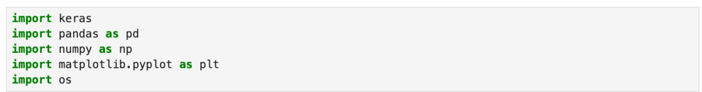
Key Python libraries used in this exercise are:

• Keras
• Pandas
• Tensorflow
• Maplotlib
• sklearn

Model Code

The notebook with this code can be accessed here: https://anaconda.cloud/share/notebooks/b75a2847-4d92-4727-a36a-95ad898e8aa6/overview

Let us start by importing required libraries. Depending on your version of Python and Tensorflow, you may run into few warnings. Make sure you read those warnings to ensure that none of it will impact your model building exercise.

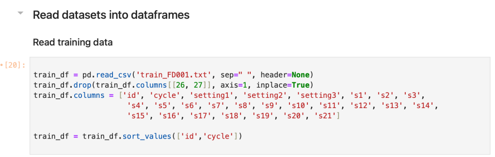
As you can see above, I have also set up seed for reproducibility in one of the code snippets above. Now that we are done importing the libraries, let us read our data sets.

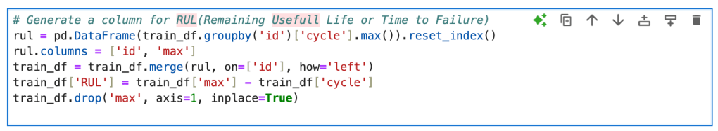
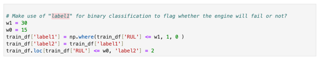
Next, we get into data labeling. We start by creating a column for Remaining Useful Life (RUL)

Then, we generate column labels for the training data.

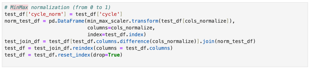
After creating those labels, we get into data normalization.

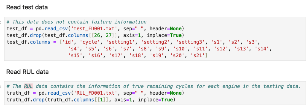
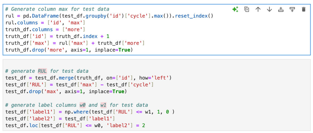
Now as a final step before we jump into building the LSTM network, we will leverage the life cycle dataset created from the RUL data to generate labels for the test data.

Now let us start building the LSTM model. First, we reshape features for LSTM. We define a function for reshaping features into samples, timestamps and features.

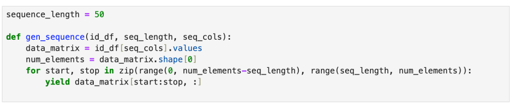
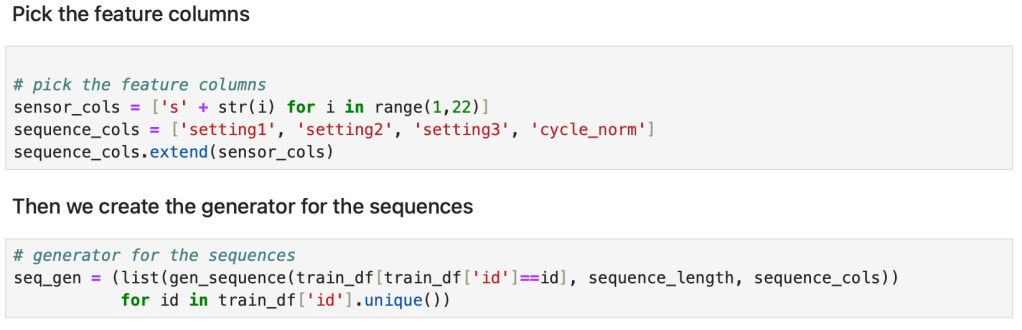
Next we pick the feature columns and then build a generator for the sequences.

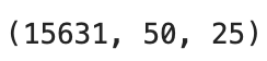
Having built the generator, let us put that to use and generate sequences. Then we convert the sequences to numpy array.

You should see the shape of the array as the output.

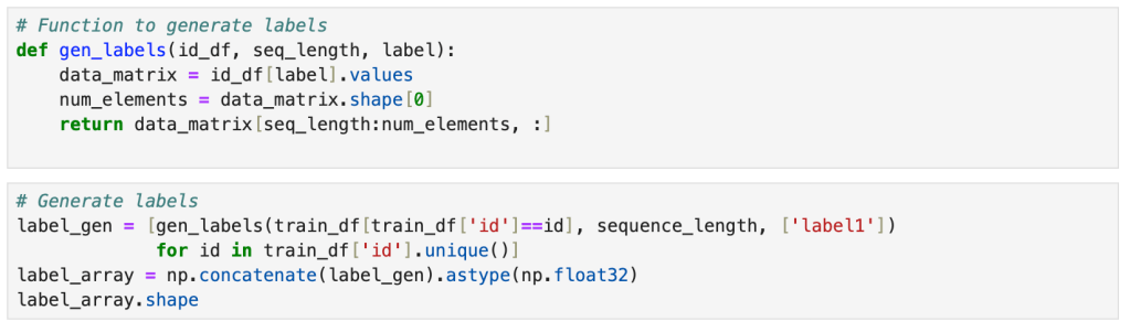
Next, we create a function to generate labels and then use that function to generate labels.

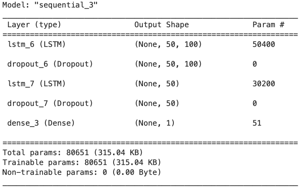
The first layer in our network is an LSTM layer with 500 units followed by another LSTM layer with 100 units. We are applying dropout after each LSTM layer to manage overfitting. Our final layer is a dense output layer. It is a layer with single unit and sigmoid activation since this is a binary classification problem.

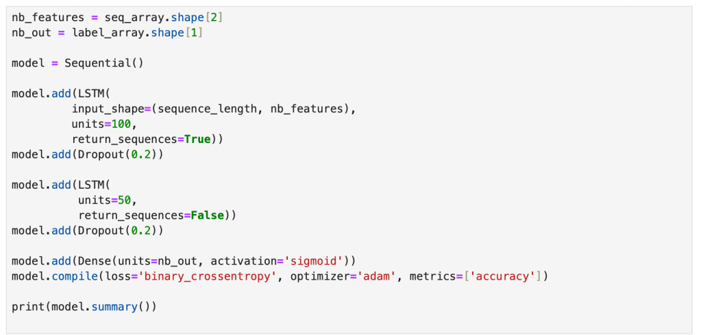
You should be able to see the model summary, like the one shown below:

The moment of truth has arrived and now it is time to fit the network. I like watching the epoch count increase. Here is a video snippet from when network fitting was underway (20X speed).

Now that the fitting part is done, let us summarize the data to understand model accuracy. The code that we will use is shown below.

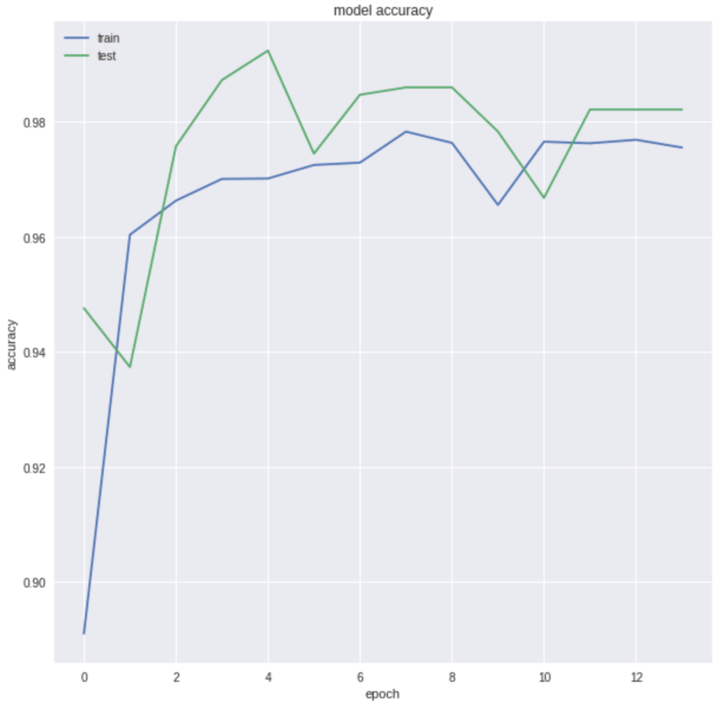
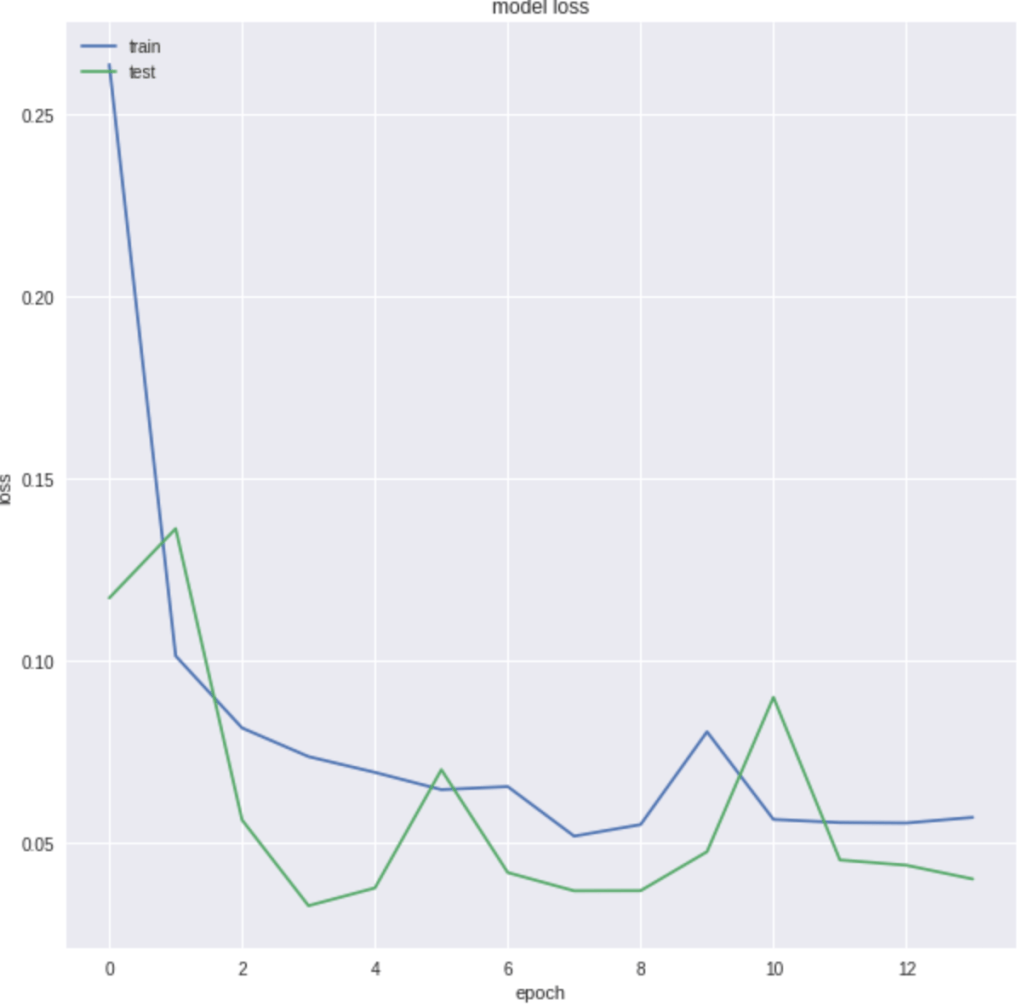
The graph generated shows the accuracy for the training and test data and you can see that they start aligning as the epochs increase. The same goes for model loss shown below:

Let us review training metrics, starting with accuracy. As you can see, the accuracy is 0.98 (rounded).

Next we make prediction and build a confusion matrix for the same.

The output is shown below.

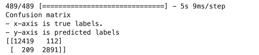
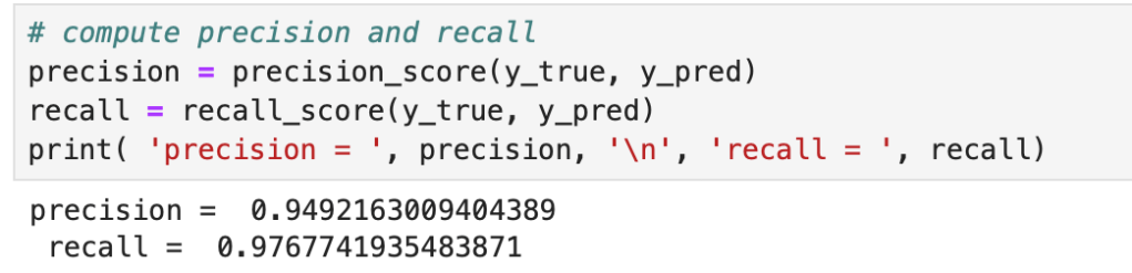
Now that we have the confusion matrix, let us calculate precision and recall.

I hope you enjoyed building this network as much as I did. Unfortunately, I did not get time today to evaluate the model on a validation set but once I do that, I will probably come back and update this post.