Predictive Maintenance With LSTMs (Part I of II)

Back in December, I wrote a two-part article on why deep learning-based algorithms are better suited for predictive maintenance analytics. You can refer to the article, Deep Learning in Predictive Maintenance, on this blog. In the second part of this article series, I mentioned some toying around that I was doing in this area. This two-part article is a result of that. We will essentially build an LSTM-based predictive analytics model. The topic of LSTMs has been extensively covered in many of my video series, like Edge AI Bytes, GenAI Bytes and Deep Learning with Python.

We will undertake the journey to leverage LSTMs for predictive maintenance in two parts. The first part will overview why LSTMs are a good candidate for predictive maintenance. We will understand the dataset that we plan to use (NASA Turbofan Dataset) and perform exploratory analytics on the data. In the second and final part, to be published on 04/20, we will overview the code for the LSTM predictive maintenance model on this data and analyze the results.

LSTM for Predictive Maintenance

Before we build the model, let us try to understand what LSTM networks are and why they are a good fit for predictive maintenance analytics. LSTMs are a type of Recurrent Neural Network (RNN). RNNs are a perfect fit for tasks involving sequence (like words in a sentence) and because of that, they are instrumental in areas like machine translation. However, one drawback that standard RNNs have is the vanishing gradient problem.

To simplify that jargon, the weights do not get updatedh vanishing grad in networks witients, and hence the network can not learn. This leads to a decrease in performance. LSTM architecture addresses the drawback. LSTMs leverage a gating mechanism to control the flow of information and gradients.

LSTMs build the next state by replicating the previous state and then adding or removing information as required. In technical parlance, the mechanisms of adding and removing information are called gates. As you may have interpreted from the overview covered in many of my video series, LSTM is a great fit for time series predictions. The primary reason behind this fit is the ability to remember previous inputs for long durations. This capability allows LSTMs to handle sequences with long-term dependencies. In simple terms, “long-term dependencies” means instances where earlier time steps may significantly impact later time steps. And if you think about the streaming data being continuously generated and transmitted by sensors, it fits the bill.

With this background, let us jump into building a predictive maintenance model using LSTMs.

Data set

Data used for this exercise is NASA’s turbofan data. The details of this dataset, as shared on the dataset page linked above, is below:

Data sets consists of multiple multivariate time series. Each data set is further divided into training and test subsets. Each time series is from a different engine i.e., the data can be considered to be from a fleet of engines of the same type. Each engine starts with different degrees of initial wear and manufacturing variation which is unknown to the user.

This wear and variation is considered normal, i.e., it is not considered a fault condition. There are three operational settings that have a substantial effect on engine performance. These settings are also included in the data. The data is contaminated with sensor noise.

The engine is operating normally at the start of each time series, and develops a fault at some point during the series. In the training set, the fault grows in magnitude until system failure. In the test set, the time series ends some time prior to system failure. The objective of the competition is to predict the number of remaining operational cycles before failure in the test set, i.e., the number of operational cycles after the last cycle that the engine will continue to operate. Also provided a vector of true Remaining Useful Life (RUL) values for the test data.

The data are provided as a zip-compressed text file with 26 columns of numbers, separated by spaces. Each row is a snapshot of data taken during a single operational cycle, each column is a different variable. The columns correspond to:
1) unit number
2) time, in cycles
3) operational setting 1
4) operational setting 2
5) operational setting 3
6-26) sensor measurement 1-26

Data Set: FD001
Train trjectories: 100
Test trajectories: 100
Conditions: ONE (Sea Level)
Fault Modes: ONE (HPC Degradation)

Data Set: FD002
Train trjectories: 260
Test trajectories: 259
Conditions: SIX
Fault Modes: ONE (HPC Degradation)

Data Set: FD003
Train trjectories: 100
Test trajectories: 100
Conditions: ONE (Sea Level)
Fault Modes: TWO (HPC Degradation, Fan Degradation)

Data Set: FD004
Train trjectories: 248
Test trajectories: 249
Conditions: SIX
Fault Modes: TWO (HPC Degradation, Fan Degradation)

With that note, let us start exploring the key steps involved in building the LSTM model.

Exploring NASA Turbofan Data

Before we do a deep dive into building an LSTM model, let us explore the dataset to understand it. This exploratory phase also helps decipher the results later on. We will also build a baseline regression model for the data in this part. You can download the notebook from this link:

https://anaconda.cloud/share/notebooks/3c9fa7bd-feb5-436f-b21d-01e5155a94d1/overview

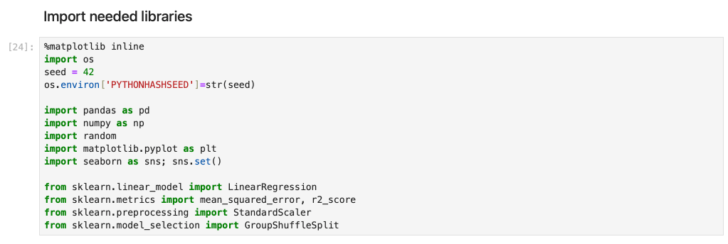
We begin my importing the needed libraries

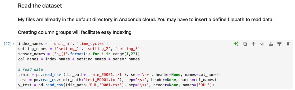
Then read the dataset. Make sure you define the path if the files are not in your default directory. Also, at this point, you can create groups of columns to facilitate easy Indexing later.

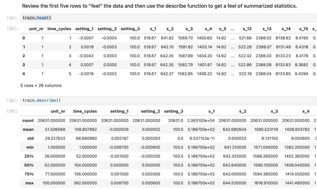
Review the first five rows to “feel” the data and then use the describe function to get a feel of summarized statistics.

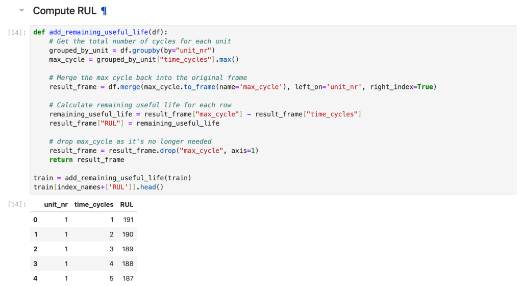
Next, we will build a RUL indicator. In case you are not familiar with the RUL metric, RUL stands for Remaining useful life. It is the length of time a machine will operate before it breakdowns, requires some form of repair or replacement. By calculating RUL, maintenance professionals can schedule maintenance, optimize operating efficiency, and mitigate unplanned downtime. Because of these reasons, RUL is one of the top metrics in predictive maintenance domain.

There are few different ways to calculate RUL metric. Examples are:

Leveraging lifetime data
Run to failure data
Threshold data

In our dataset, RUL is the number of flights remaining for the engine after the last datapoint in the test dataset. Let us define a function to compute the RUL.

We can view the distribution of the RUL data using this code snippet.

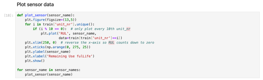
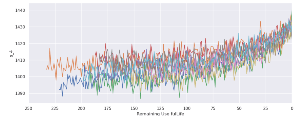
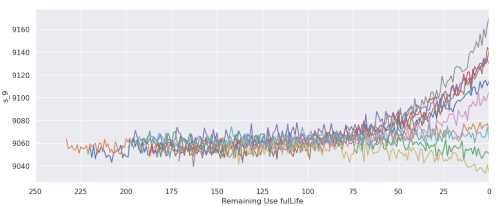
Next, we explore the sensor data by plotting it. The code snippet below does that for us. Below the snippet you can see the examples of the graphs that the code generates. As you can see, we want to visualize sensor data over the RUL.