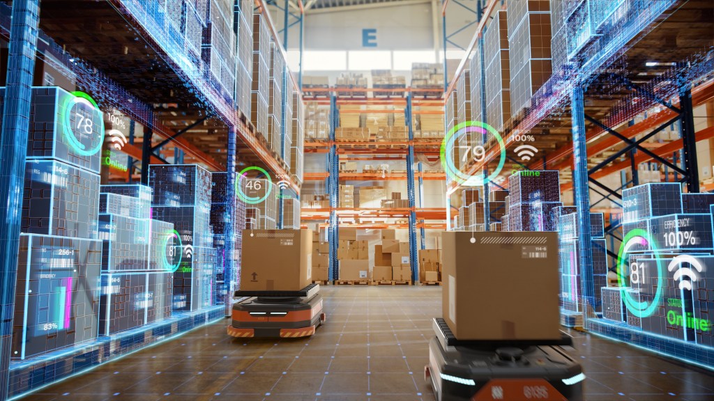
Back on October of 2018, I wrote a short story on a blogsite I used to manage, focusing on AI-enabled supply chain planning. It was the era of the initial avatars of Generative AI but you could see the writing on the wall. I predicted that this story happens in 2029. Looks like this will be reality by then.

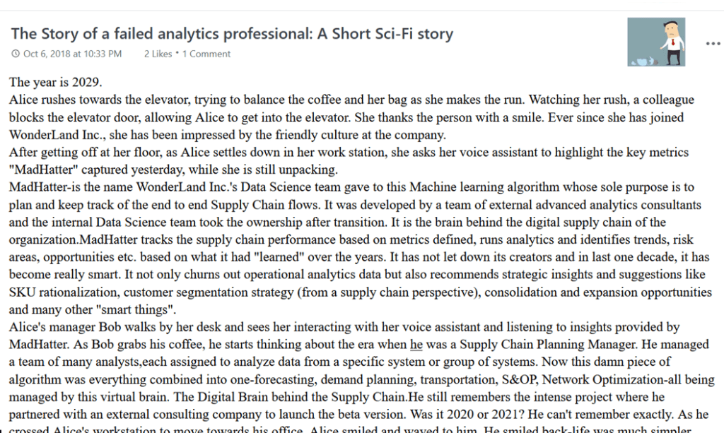
Review the text from the story in the screengrab below. If you are conversant with recent Generative AI models, you know that you can actually train Generative models to achieve these tasks.

In a video I posted on LinkedIn on 5/24, I postulated that within next 5 years, Generative AI models will be leveraged extensively in supply chains, and given the pace of technology, and the scope of applications, that is a given. So add five years to 2023 and the 2029 prediction is certain to be a reality in 2023.

The secret sauce with success in technology domain is not which technology you use. It is understanding what path the technology will take, how it can be leveraged and how it will impact business landscape in next 5-10 years. Consider this- Microsoft funded OpenAI took the lead in Generative AI race but it does not stop any company to reap the benefits. The value of this technology is in the value it creates being part of the solutions.

And you do not need to wait 5 years to explore the value.

You can start experimenting as well as embedding Generative AI in your overall AI strategy.

This post summarizes an attempt to mimic what a “real-time” supply chain planning algorithm may look like structurally, in production. And to be honest, while this was an interesting experiment, this is already obsolete. You can train Generative AI to build these models learning from your data. But for nerdy fun, let us start with briefly stating our objective:

To address the possibility that artificial neural networks can help predict the capacity of the simulated supply chain network to fulfill incoming orders for the next upcoming period. This experiment combined a multi-echelon supply chain simulation model with an artificial neural network architecture.

To keep the experiment simple, our supply chain handles only one product and consists of four echelons: supplier, production, distribution, and retailer. The time between order arrivals is fixed and set with a length of the one-time unit.

We create a random demand data set where the order size is variable and follows a normal distribution with a mean of 40 units and a standard deviation of 2 units. The values of these parameters were selected along with a set of other parameters related to the four nodes:

• Re-order points,
• Quantities to order upstream
• Transportation times between nodes
• Transportation capacities for the four nodes.

The Approach

In the simulation model created for the supply chain described above, parameters were adjusted using successive iterations until the service level in the retailer was around 90%, and the service levels on the other nodes of the SC were also balanced around the same values.

Model Architecture

The retailer is the entity in charge of fulfilling the orders. When the re-order point is reached, an order is placed towards the distribution center to refill the inventory. The replenishment sent from the distribution center is a fixed quantity. If a backorder occurs (the current inventory is insufficient to satisfy the order), the available quantity is sent immediately, and the rest is dispatched as soon as its inventory is loaded.

Replenishment policy

The ordering policy used is the order point, order quantity so-called (s, Q) system, in which both re-order point, s, and order quantity, Q, are fixed.

It is a continuous review policy to provide a stable service level, although it does not cope effectively with sudden large orders. The same procedure is applied through all the nodes, i.e., the orders from the distribution, production, and supplier are sent to their respective upstream node, induced by inventory levels lower than the corresponding re-order point.

The echelons are connected through a transport mode set with a restricted capacity and fixed transportation time. Moreover, warehouses are assumed to have unlimited storage capacity, and at the beginning of the Supply Chain, there is an entity holding enough inventory capable of feeding the supplier.

All these settings infer that the uncertainty in the SC comes from the size of the orders that the retailer must deliver.

Regarding the outputs, it was registered the time in the system of each order and the inventory levels of each echelon whenever a new order entered into the system

The Neural Network Model

A a multi-layer perceptron set with one hidden layer, was created for this experiment. Multi-layer perceptron is the most common type of neural network for networks with three layers or more (n ≥ 3):

• One input layer,
• One output layer and
• One or more hidden layers.

The weights connect neurons from consecutive layers, and these connections exhibit different values according to the importance perceived after the iteration process in the training phase.

As mentioned in one of the previous sections, the artificial neural network was fed with data generated in simulation runs. The number of neurons in the input and output layers were not fixed: they were re-adjusted considering the past and future boundaries using Python programming.

After training the network, the test phase was performed with untrained data, and the recognition rates were calculated by comparing the outcomes (outputs) with the values returned from the simulation.

The architecture of  both experiments

In experiment 1, the goal was to anticipate the capacity to dispatch instantaneously the upcoming orders. In other words, the time the order stays in the system is zero if the inventory at the retailer is sufficient to fulfill that order and more significant than zero otherwise, which means that it was not satisfied immediately (retailer stock out).

It is possible to identify the expected time to fulfill the orders accurately. The variable p represents the prediction time horizon. The output layer has different lengths depending on the number of periods, p, to predict.

In experiment 2, the entities that reach their re-order point place a new order upstream. The network can foresee when and in which nodes these situations will happen. As stated before, the inputs represent the inventory levels of each entity. To organize the targets, the values were set in groups of five neurons, in which the first four are activated when their respective entity reaches the re-order point.

In this case, each neuron represents one different echelon. N1 will turn to 1 if the inventory level on the retailer is expected to be below the re-order point, and the same for the neurons N2, N3, and N4, pertaining to the distribution, production, and supplier nodes, respectively.

A fifth neuron will act as a control neuron, and it is activated when none of the other neurons were activated in that period.

For both experiments, the inputs are the same. The neurons N1, N2, N3, and N4 represent the inventory levels of each SC node, retailer, distribution, production, and supplier, respectively. The input layer can either be set considering only the inventory levels of the instant t when an order arrives in the system or extending the period considering historical data.

In this case, the input layer is set with all inventory levels from the instant t to the instant t – q + 1, where q represents the number of periods considered.

Experiments and results

The sample used to train the artificial neural network comprised the information of 216000 different periods generated by the simulator. The tests were performed with a sample with data regarding 24000 periods generated with different runs from untrained data.

Conclusion

Regarding experiment 1, the outcomes were remarkable: the recognition rate was more significant than 99.5% for predictions for the next period and over 98% for forecasts for the three subsequent periods. These results were compared with a new experiment, using as input only the information on the inventory level in the retailer. In that experiment, the recognition rate for more significant periods was lower, which proved that visibility in supply chains is essential and increases prediction accuracy. In experiment 2, the results were 97% for predictions for the next period and 75% for a time horizon of three periods. As the period is enlarged, the recognition rate decreases by 10-15% for each added period.

Moreover, we can conclude that it is irrelevant to extend substantially the historical data once the outcomes when using only two periods (the current and the previous periods) are practically the same compared with the results from more significant periods.

Therefore, we can conclude that artificial neural networks can be used to effectively predict potential disruptions in supply chains more accurately than conventional planning methods.

My next steps for modifying this algorithm are to (1) introduce complexity in the SC model by adding new nodes, types of products, and additional sources of uncertainty like variability in transportation times, transportation capacities, and the processing time in each entity, and (2) perform the same challenges but using a smaller sample size to train the network and use recurrent neural networks to cover that complexity.