Optimizing tactical manufacturing operations generally minimizes or maximizes certain measures to enhance process efficiency, quality, and productivity. While these optimizations eventually lead to reduced costs and enhanced customer experience, smart manufacturing should allow us to directly tie every tactical manufacturing decision to profitability.

The current state and its drawback

Let us use a hypothetical example of a footwear manufacturing company. We have the data from their shoe buckle manufacturing line. This line manufactures steel buckles of all sizes for many shoe lines for both men and women. The cost explanation for this manufacturing setup is in the appendix section (Appendix B). We will focus on this line, which is a cutting operation, to discuss our proposed expert system algorithm.

One of the key decision points for such a line is identifying a feasible range of system parameters. For this type of line, the priority is generally given to the determination of possible ranges of three cutting parameters to assure the product quality:

• Cutting speed
• Feed
• Depth of cut

Afterward, alternative plans may be formed within the identified feasible ranges to guarantee that these alternative plans are meaningful and practical. The final method that is eventually selected for a given part number will be a function of a pre-determined goal.

With a smart factory setup, manufacturing planning is not only a matter of core operations data. Cost analysis to evaluate the variable and fixed costs associated with manufacturing operations is critical to a good plan. The planning should also be related to making an appraisal to justify possible technical and economic benefits of adopting new manufacturing technologies. Smart manufacturing allows you to tie your tactical decisions with costs.

The Architecture for the Simulation Experiment

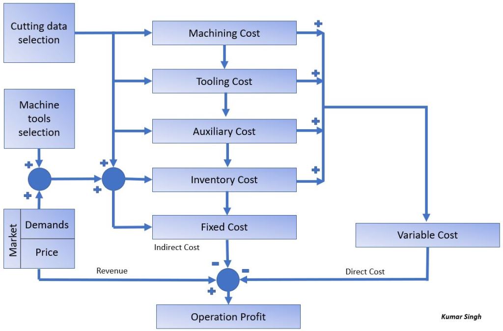
The figure below shows the high-level structure of my proposed solution. I made something up for the experiment for any data . The first element in the architecture is a classic scenario generator, like the ones you have in simulation models, which is built on the manufacturing system to provide qualified plans. The second element is a cost analyzer to identify and evaluate fixed and variable cost components. The third element is an optimizer to select the optimal strategy based on the prescribed criterion from the management. The 4th component, as illustrated in the diagram below, is the comparator which tests the optimality and assesses the validity of adopting new and advanced machining operations from an economic perspective.

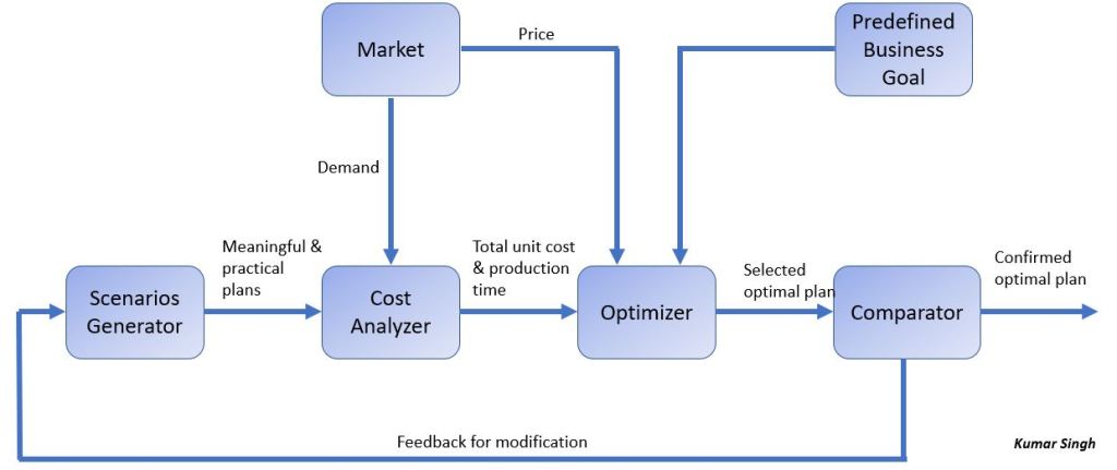
The feedback path from the comparator to the alternative generator determines the direction and amount of change in the three cutting parameters for improvement, and this closes the optimizing loop. The loop will then interact with the surrounding environment through the market, which evaluates the demand and price of the part to be machined. The corresponding system dynamics diagram is below:

Applying the Theory to Real Life

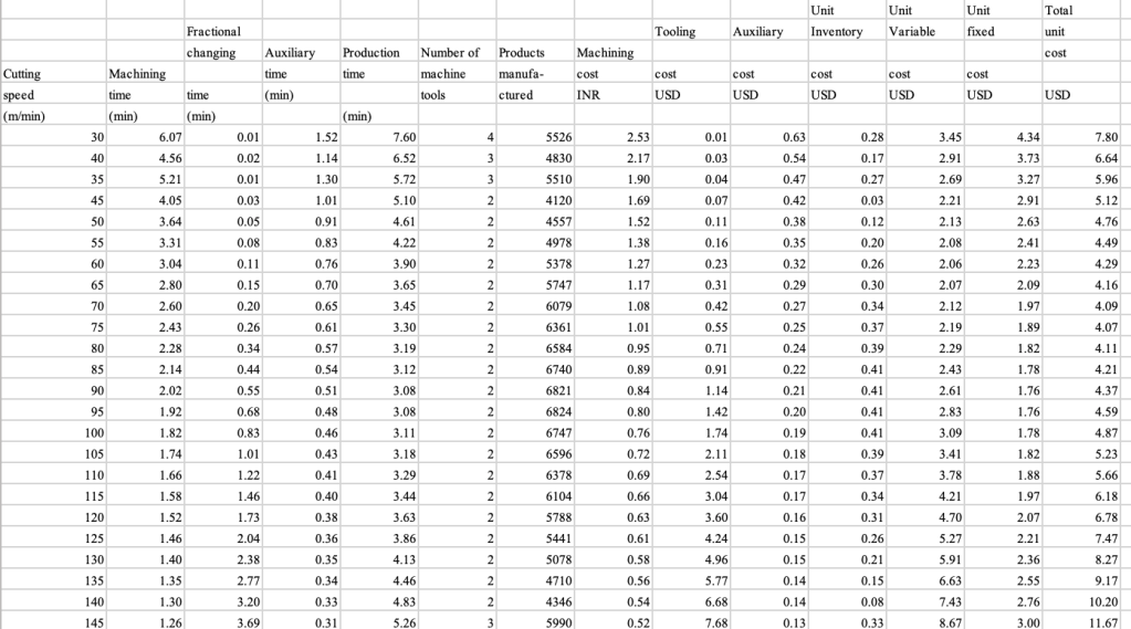
A sample of the data from the buckle line .

The critical relationships among various parameters have been shown in the graph below.

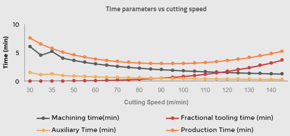
This graph captures relationships between production time as a function of machining time, fractional tooling time, and auxiliary time. Fundamental relationships are summarized below. I would like to see what other granular relations you can find from the attached data.

Relation between production time and cutting speed

The production time fluctuates as the cutting speed varies from 30 m/min to 145 m/min. It reaches its minimum value of 3.08 min/piece at a 95 m/min cutting rate. If the first five columns of data in our table are observed, as shown in the graph below, the machining time decreases significantly as the cutting speed grows. However, with the same increase in cutting speed, the fractional Tool changing time needed for maintaining a workable cutting edge during machining increases accordingly.

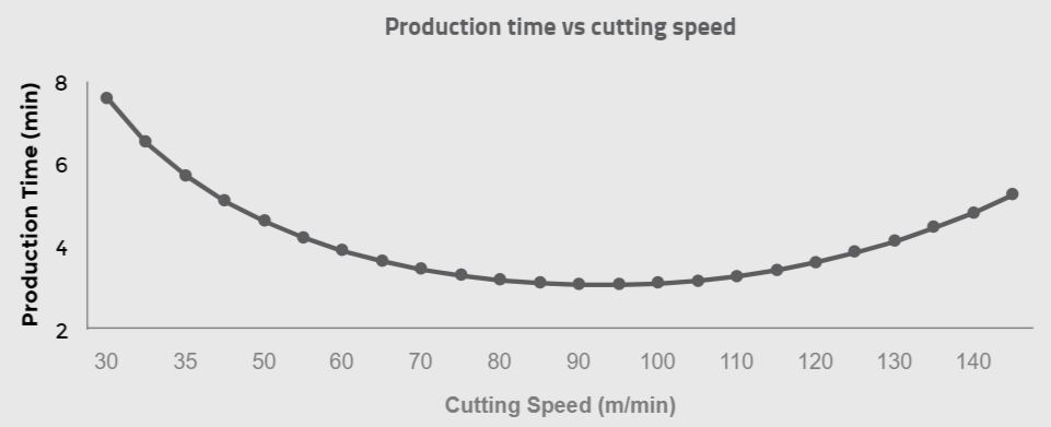
The primary driver for this is the short tool life resulting from the high speed at which the cutting machine operates. As you can interpolate, the minimum production time is a balancing act between the machining time and the fractional Tool changing time, and both of these parameters are functions of the machine’s cutting speed.

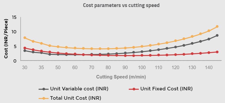
Relation between Total Unit cost and cutting speed

Before you go further, please refer to the primer on cost calculations used in the experiment in the appendix of this post.

The total unit cost also varies as the cutting speed increases from 30 m/min to 145 m/min. It reaches its minimum INR 4.07/piece value at cutting speed = 75 m/min. The drivers behind this are:

• A lower unit fixed cost than those produced at cutting speeds lower than 75m/min. This cost is listed as  INR 1.89/piece.
• A lower unit viable cost as compared to those produced at cutting speeds higher than 75 m/min. This cost is listed as INR 2.19/piece.

Relation between operating profit and cutting speed

A significant goal of manufacturing is to support the organization in attaining profits. A dynamic system example of the role of profit during manufacturing operations and the cost analysis of the experiment is shown below in the form of a graph.

———————————————————————————————————————————

Appendix A: Our case study example

If you are a manufacturing professional, you know that cutting speed plays a significant role in both quality of machined parts and machining tools. This case study will analyze the cost and productivity of machining operations run under different cutting speeds. The parameters for our case study are:

Workpiece

• Material: AISI 1035 steel
• Diameter 56mm (initial)  60mm (final)
• Length: 250mm

Tooling

• Material: Carbide
• (tr and vr): (100 min, 80 m/min)
• exponent n: 0.2
• Tool cost: USD 25/piece
• Changing time: 15 min

Machine Tool

• Capacity: 175 hours/month
• Fixed Cost: USD 6000/month

Cutting data:

• d limit: 2mm
• Feed: 0.25 mm/rev
• Auxiliary Time: 25% (Machining time)

Managerial Data:

• Monthly Demand: 4000 pieces
• Wage Rate:USD15/hr
• Overhead: USD10/hour
• Holding Cost: USD 1/piece
• Revenue: USD 9/piece

Appendix B: Identifying relationships to costs:

MT = Machine Time

PT = Production time

TL = Tool Life

Machining Cost = (Wage Rate + Overhead) X MT

Tooling Cost = MT/TL x (Tool Cost) + MT/TL x (Changing Time) x (Ware Rate + Overhead)

Auxiliary Cost = (Wage Rate + Overhead) x (Auxiliary Time)

Inventory Cost = Holding Cost [ ((No of Machines)(Capacity Hours) x 60)/PT – Monthly Demand]

where Production Time = PT = MT + MT/TL x (Changing time) + Auxiliary Time

Unit Inventory Cost = Inventory Cost / ((No. of Machines)(Capacity Hours) X 60 /PT)