Traditional Inventory Optimization (IO) and Multi-Echelon Inventory Optimization (MEIO) algorithms identify cost savings opportunities based entirely on Inventory stored at specific locations. Essentially, the algorithm aggregates the SKU/Product group inventory for that location.

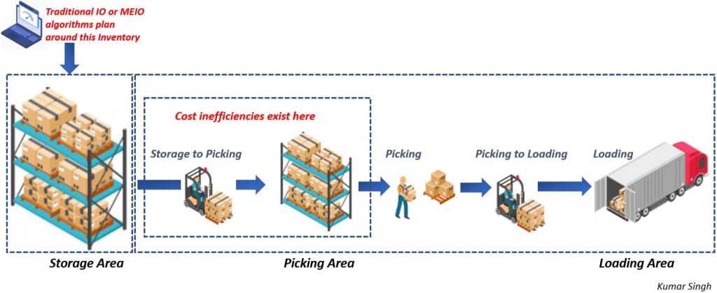
While it still generates value, a significant gap remains. Such decisions may impact the optimality of warehouse operations. Reduction in the storage inventory of a product group may mean frequent replenishments from storage to the picking area, thereby increasing operating costs or increasing the probability of late or missed deliveries to the customers, as shown in the illustration below.

One of the handicaps of not making IO or MEIO more granular was the solver run time these models usually take. We are now well-positioned to start experimenting with adding more granularity to the concept. Using open-source tools and granular warehouse processes data, we can develop an underlying foundation optimization model that takes the concept of Inventory optimization to the shop floor.

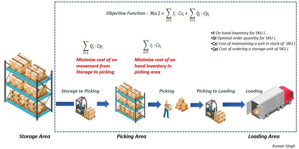
This proposed model takes Inventory Optimization to a whole other level of granularity. It essentially manages the Inventory in the picking area and picking process optimally, thereby minimizing total picking area warehouse optimization cost. This is based on an experiment done with a sample data set. It works on the toy data set so you can try using this approach with real-world data.

Such a model can be foundation for generating millions to scenario to train a deep learning model as well. But for now, let us focus on the topic at hand.

The first illustration essentially shows how Inventory Optimization is typically done today. It takes into account only the Inventory in storage at warehouses.

This proposed model, takes Inventory Optimization to a whole another level of granularity. It essentially manages the Inventory in the picking area and picking process optimally, thereby minimizing total picking area warehouse optimization cost.

The Picking Process

Before we jump into the model structure, we will walk through the generic picking process at a high level to better understand the nuances of the model.

Storage to picking

The supply process is carried out systematically but not for the same reference. When a product is about to go out of stock or has been entirely out of stock, it proceeds to request storage transport using a forklift from the corresponding rack to be supplied with the picking shelves.

Fulfillment request

Once any of the points of a sale send the record of the sales made of any product, a request for supply of that specific SKU (Stock Keeping Unit) and the quantity arrives.

Pickup Request

This data is registered in the technology platform of the pickers indicating this information to supply this product at the specific point of sale; by using a container that will have the products requested by a store, the operator proceeds to collect these items.

Pickup to loading

When the container is ready, the process of labeling is carried out with the supplied information about the products, as well as the destination; they are then taken to the loading area, where they will be waiting to be transported to the different points distributed in other cities of the country.

Model Structure

Decision Variables

• Ii On hand inventory for SKU i.
• Qi Optimal order quantity for SKU i.

Parameters

• Ci Maximum warehouse capacity for SKU i
• Csi Cost of maintaining a unit in stock of  SKU i
• Cpi Cost of ordering a storage unit of SKU i
• Li Inbound Transportation lead time of the SKU i
• Iii The beginning Inventory of SKU I in the picking area
• Di Daily demand for SKU i
• SSi Safety stock of SKU i

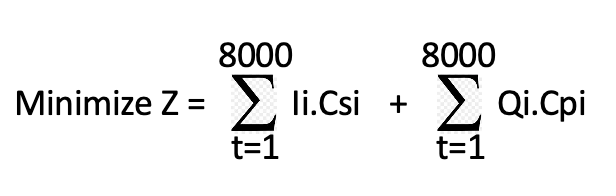
Objective function:

Minimize the total cost of the organization during the planning horizon. In this case, it is one day. The total number of SKUs in the data I used for my pilot was 8000.

Constraints:

The productivity of the workforce: The workforce’s productivity is defined as the relationship between time, work time, delivery time, and the number of units ordered. The working day is 8 hours daily.

Inventory: The Inventory of the reference I must be equal to the Inventory in the immediately previous period, plus the order size made in that period, minus the required amount, and minus the Inventory that must remain in stock to guarantee the production flow.

Picking capacity: The number of daily units in Inventory cannot exceed the ability of the picking area.

Security stock: The daily units in the Inventory of reference cannot be less than the security stock.

Constrain positive: Ensure that the variables take positive values.

Stages of Model Formulation

The construction of the model went through several stages; these are described in detail below:

Stage 1: Gathering the necessary information for the implementation of the model correctly as historical demand, in-place Inventory for each reference, storage capacity in picking, and distance from the stock storage area to the corresponding picking storage area.

Some examples of challenging data points are in the appendix

Stage 2: Based on the data found, we proceed to determine the following:

• the costs of maintaining the units in Inventory,
• of making an order and the waiting time to supply, and
• The lead time of the product, with which we proceeded to calculate the minimum-security stock to have a 95% service level.

Stage 3: Through linear programming, a supply planning model was built, with the Solver tool in which the decision variables were established, such as the optimal quantity of inventory, order size, restrictions of maximum inventory capacity, productivity, and minimum level of inventory whose objective is to minimize the costs of the operation of supply and storage in picking.

• Ii: Optimal on-hand units in the Inventory of each SKU
• Qi: Optimal order size for each SKU
• SSi: Safety Stock, the minimum level of Inventory that allows meeting the customer’s demand with a service level of 95%. A value of k and d of 1.64 for a normal distribution corresponds to this percentage.
• Li: Lead time is the time that elapses between the order being placed and the delivery of the order.
• Restriction on Inventory: This restriction guarantees the customer’s demand is 100% satisfied.
• Restriction on Capacity: This restriction ensures that the units in the Inventory do not exceed the maximum capacity of the distribution center.
• Restriction on productivity: This restriction ensures that the productivity goals will be met within the available times of the working day.

Appendix: Sample list of required data points

ABC: Classification of products in categories ABC according to the reference’s rotation.
Product Location: Coordinates the product location in the distribution center as its respective one; sector, hall, level, rack, and position.
Sector: Zone of the warehouse to which it belongs.
Hall: The hall in which the shelf is located.
Level: The rack level it is found is numbered from 1, which is the closest to the ground.
Rack: Subdivision of the shelf where it is located
Position: Specific position of the product inside the cubicle
BUO: Basic ordering unit.
Available: Units of the product in the storage area.
Demand: Units demanded by the client; information of its historical data granted by the company.
Daily demand +desviation: It is equivalent to the daily demand summation of said reference plus the deviation of that demand.
Daily demand destination is the deviation of the daily demand for that product.
Reorder: This point indicates when the order must be placed in hours or days of optimal Inventory using the tool Solver = Ii/Di  Order: Q Is the optimal order size for each reference. This value is extracted from running the optimal supply model utilizing the solver tool. To this item belong the following four columns: Hour, Days, Q, and Shelving. Q = Qi
Hour: Duration of Inventory in stock in hours. = Inventory on hand units/(Demand + Deviation units/8 (hr))

Days: Duration of the Inventory in stock in days
Q: Corresponds to the optimal order size for each reference. This value is extracted from the execution of the optimal supply model utilizing the Solver tool.
Shelving: Round the order size Q, according to the multiple of the BUO.

Available/Hour inventory: Equivalent to the product among the reference units on the shelf for the hours of Inventory on Shelving = Available x Hour/Shelving

Demand/Hour inventory: It is equivalent to the product between the daily demand and the deviation from the reference for the hours of duration of the Inventory on Shelving, all the above about 8 hours a day of the working day = ((Daily demand + deviation x hour)/Shelving)/8
Horizon: In this, the working days of the week are divided into 4-time slots of three hours each, and the units in stock were calculated with the following conditional equation.

AV/Hours <= Reorder (Hours); Order (hours) + AV/Hours -(Demand x3)

AV/Hours >= Reorder (Hours) ; AV/Hours -(Demand x3)

Logistic operator direct workforce cost.

Forklift cost

Ordering costs